Maximum Power Transfer

In this experiment we study the concept of maximum power transfer within a circuit, and use this theorem to determine the Thevenin resistance of such circuit. The Maximum Power Transfer states that maximum power from circuit to resistive load will be achieved once load resistance = Rth.

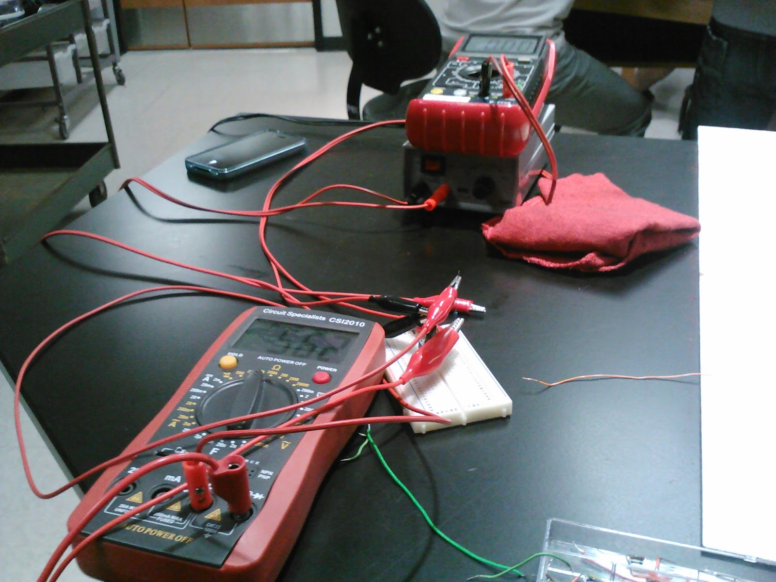
First the following circuit is constructed:

where R0 is a variable resistor, in this case a potentiometer

	Nominal	Measured
Resistor	5.6 Kohm	5.62+/-.02 Kohm
Voltage source	4.5 V	4.54 V

The potentiometer was varied so that we could get readings of voltage and resistance coming from a wire attached to the potentiometer. 

After getting values for voltage and resistance, we can compute the power through the potentiometer.

Measured V0 (V)	Measured Rx (Kohms)	Calculated P0 (W)
2.80+/-.01	14.64+/-.01	0.000536+/-.0000028
2.68+/-.02	13.73+/-.01	0.000523+/-.0000055
2.51+/-.01	12.55+/-.02	0.000502+/-.0000029
2.43+/-.01	12.08+/-.01	0.000488+/-.0000028
2.32+/-.02	11.50+/-.01	0.000468+/-.0000058
2.17+/-.01	10.77+/-.01	0.000437+/-.0000029
1.98+/-.01	10.00+/-.01	0.000392+/-.0000028
1.80+/-.02	9.34+/-.01	0.000347+/-.0000055
1.63+/-.02	8.78+/-.02	0.000303+/-.0000053
1.41+/-.01	8.17+/-.02	0.000244+/-.0000025
1.28+/-.01	7.82+/-.01	0.000210+/-.0000023
0.84+/-.01	6.89+/-.01	0.000103+/-0000017
.02+/-.01	5.65+/-.02	0.00000007+/-.00000
.00+/-.001	5.62+/-.02	~0

Analyzing the Thevenin equivalent circuit, we can calculate the theoretical voltage and power going through the potentiometer using voltage division;

where x is the value at which the potentiometer is set for every voltage.

Theoretical V0 (V)	Theoretical Power (W)
3.25	0.000721
3.20	0.000746
3.11	0.000771
3.07	0.000780
3.03	0.000798
2.96	0.000814
2.88	0.000829
2.81	0.000845
2.75	0.000861
2.67	0.000873
2.62	0.000878
2.48	0.000893
2.26	0.000904
2.25	0.000901

Looking at Fig. 2, we can observe that:

Max Power (0.536KW) occurs at 14.64kohms.

To get the theoretical value of the resistance at which max. power occurs, we solve for R in P = v^2/R, where the voltage is 2.80V (voltage at which max. power happens);

R = 2.80^2/0.000536 = 14626.87 ohms

% Error = 0.137%

Part B:

For the second part of this experiment we used Logger Pro software to obtain a graph of power. The circuit, however, was a little bit more complex;

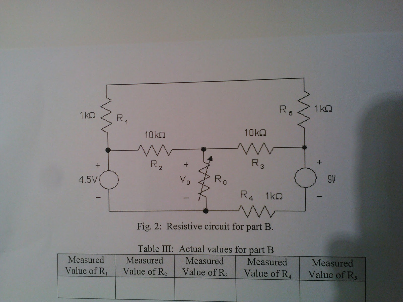
	Nominal (kohms)	Measured (kohms)
R1	1	0.966
R2	10	9.85
R3	10	9.86
R4	1	0.976
R5	1	0.979

	Nominal (V)	Measured (V)
Voltage source 1	4.5	4.54+/-.01
Voltage source 2	9	9.05+/-.01

Logger Pro Graph Power vs. T

The power graph was obtained by dictating a function that multiplies voltage and current. Unfortunately, the graphs for voltage and current were less than satisfactory due to the amount of error and the sensitivity of the probes.

Notice the spikes on the voltage graph

This results compromised the data analysis for this part.