Tuesday, May 21, 2013

FREEMAT - Complex Numbers

Assignment


Matrix Problem;


MOSFET Control of an Electric Motor Lab

For this lab we studied the behavior of a motor which basically is an inductor with magnets inside that reacts to voltage input.

We used a function generator as well as an oscilloscope to obtain graphs.

Flyback Voltage
In the first part we tested flyback voltage which consisted on just the motor and a 2.2 Kohm resistor.

We set up the oscilloscope for single sweep with vertical scale of 10v/div and time scale of 0.1 ms/div.

We obtained the following graph:


A 1N4007 diode was adapted to the circuit so that it could correct the noise in the graph.


We noticed that even with the diode, we could still see the flaws on the graph (eg. the sharp, uneven peaks).
We also noticed that the diode would get warm after the motor was left running for a long period of time.


Open Loop MOSFET Voltage Control Unit
On the following part, we studied the effects of adding a MOSFET transistor which it's an analog of the variable transistor; source voltage controlled resistance. The function of a MOSFET is to control the flow of current in the Source and Drain leads which is governed by the Gate voltage. We also added a potentiometer that allowed us to change the resistance, and hence vary the voltage (gate voltage of MOSFET) on the motor.


By turning the potentiometer VERY SLIGHTLY, we measured the start-up voltage of the motor to be 3.9V.

Looking at the formula;
Rds =  VdRl / (Vs-Vd)
we can see that Rl (in this case the motor), is driven by the resistance of the MOSFET. And since the MOSFET behaves as a variable resistor, we can control it via the potentiometer. We also see that when the voltage drain is smaller than the voltage source Vs, the ratio Vd/(Vs-Vd) decreases as Vd decreases.

When we attempted to slowly increase the voltage gate from zero, it was quite difficult to have steady control of the motor. The voltage was fluctuating rapidly in short periods of time.

We measured the motor DC internal resistance to be 2.5 ohms.


Part 2: PWM Chopper MOSFET Motor Control
In the last part of this experiment we analyzed how motors act when a pulse is applied to them. In a broad picture, pulses continously turn on and off the motor in a periodic matter.The motor was fed by a function generator instead of a potentiometer, and it was set to generate a square wave.


When we reduced the frequency from 10 to 6.73 Khz we noticed that the motor emitted pulses

The duty cycle of the square wave was varied from 0 to 100% resulting in the motor's rotation decrease in speed.

Looking at the waves and the motor rotation, there was clearly an addition of waves going on. 

We found the time it took for the motor to go to 100 to 0% duty cycle and reach minimum speed: ~ 1 second.

Wednesday, May 8, 2013

2ODE Activity Lab


Oscilloscope 101 Lab

In this activity we acquired experience using oscilloscope as a device to measure time varying signals.


Exercise 1; Displaying and measuring a sinusoid.
Frequency = 5kHz
Peak to peak amplitude = 5V


We found the period to be 200 micro seconds.
Our peak to peak amplitude was measured to be 5V, which were the 5 squares total
The zero to peak amplitude was 2.5V
The anticipated RMS value was 0.

We used the DMM to measure voltage values.
VDC = 0.029 +/- .0001V
VAC = 1.60+/-.01V

How does VAC compare to the scope calculations?
(1.60+/-.01)2.5  =  0.640 +/- 0.0040 ~  0.7 ~ 1/sqrt(2)

Exercise 2: Including a DC offset.
We added a +2.5V DC offset and the DC coupling looked like this:


The AC coupling looked like:


There was no major difference in DC coupling.

The values of measured voltages were:
VDC = 2.53 +/- .02V
VAC = 1.634 +/- .001 V,
which agree with the graphs above.

Exercise 3: Displaying and measuring a square wave with offset.
We changed the settings in the o-scope to measure square waves:


Using the DMM we measured the voltages;
VDC: 2.53 +/-.01V
VAC: 2.53 +/-.01V

From this graph, we can measure the Root Mean Square value;

RMS = sqrt(2.5^2 * 100/100) = 2.5

Both AC and DC coupled signals looked alike.


Exercise 4: Measuring mystery signals.

We were given the following graph:


Due to the super fast speed at which the graph was moving, the camera wasn't able to capture the whole graph.

DC Voltage = 0.20V
Frequency  = 2 kHz
Peak to peak amplitude = 4V

Capacitor Charging/Discharging Lab

In this lab we studied the function of a capacitor, and how voltage and current behave when they are connected to this passive element. A capacitor is a device that stores energy supplied by a power source. The power supply initially charges the capacitor, which can later discharge and release the stored energy.

Task1: Taking a look at the following two circuits, we can develop expressions for Vth and Rth:


a). Rth = Rcharge*Rleak/(Rcharge + Rleak)
     and
     Vth =Vcap = Rleak(Vs)/(Rleak + Rcharge)

b). Rth = Rdischarge*Rleak/(Rdischarge + Rleak)

Problem: Design, build and test a charge/discharge system with Vs = 10V power supply, charging interval 20s with resulting energy of 2.5mj, and discharges in 2s.

Step 1. Required Capacitance

w = 1/2*CV^2;        C = 2W/v^2 = 2*0.002/(9)^2 = 61.728 microF

Step 2a. Estimate value of charging resistance (ideal capacitance).
It takes about 5 time constants (tau = RC) to charge up to source voltage.

5Tau =5 RchargeC = 20s;          Rcharge = 20/5C = 20/(5 * 61.728microF) = 64.7kohms

Step 2b. Calculate peak current charge and peak power.

Icap,charge = (Vs/Rcharge)e^(-t/RchargeC) = 0.1389 A

Power = 1.2501 W

Step 3a. Estimate value of discharging capacitance.

5Tau = 5RdischargeC = 2;        Rdischarge = 2/(5C) = 2/(5*6.173*10^-5) = 6.5kohms

Step 3b. Calculate peak discharge current and power in resistor.

Icap,discharge = -(Vic/R)e^-t/RdischargeC = -1.389mA

Power = 0.0125 W

Step 4: Build the circuit.


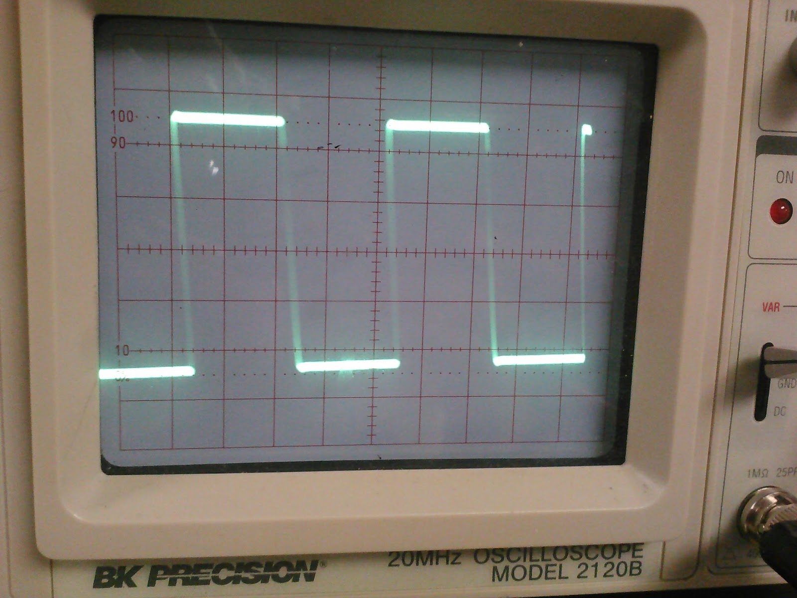
Step 5. For this experiment we used the LoggerPro interface. We used a current measuring device and a voltage prove, and hooked them up to take readings.


Charging readings:


From the graph, we can see that the final voltage achieved in the capacitor while charging was;
Vfinal = 8.523 +/- .001 V at around 18 seconds.

It's worth noting that the final voltage may not be definitive because Logger Pro saturates in this experiment, meaning that the time only goes up to 18 seconds. In reality the voltage keeps rising as time increases even if the increase is small.

Having Vfinal, we can now calculate Rleak;
Vf = Vs(Rleak/Rcharge + Rleak) = 1.15 Mohms


Discharging readings:


Based on the obtained graph, the capacitor discharged and achieved a value of 0.9 -0.7 V at around 3.1-3.3 seconds.

Step 7.
1). Calculate Thevenin equivalent voltage and resistance values seen by capacitor during charging

Vf = Vth = Vs(Rleak/(Rcharge + Rleak)) = 9*1.15*10^6/(64.7*10^3 + 1.15*10^6) = 8.521 V

Rth = Rcharge * Rleak / (Rcharge + Rleak) = 1.15*10^6 * 64.7*10^3 (1.15*10^6 + 64.7*10^3) = 61.3 kohms.


2). Calculate Thevenin equivalent voltage and resistance values seen by capacitor during discharging.
Vth = Vcap = 8.521 V


Rth = Rcharge * Rleak / (Rcharge + Rleak) = 1.15*10^6 * 64.7*10^3 (1.15*10^6 + 64.7*10^3) = 61.3 kohms.


3). At t = tau; e^-1 = 0.3679. When t = tau during charging, the voltage should be equal to 0.6321(Vf). Estimate value of tau when charging. 

0.6321*8.521 = 9(1-e^-20/tau)
0.5985 = 1-e^-20/tau
-20/tau = -0.9124
tau = 21.92

R = 21.92/(61.728*10^-6) = 355 kohms


Practical Question:
Suppose we wish to scale our result to the rail gun problem worked previously. It requires a stored electrical energy of 160MJ. The capacitor charging voltage is 15kV DC.
1. Determine required eq. capacitance

E = 1/2 CeqV^2
160*10^6 = 1/2 (15*10^3)^2 Ceq
Ceq = 1.422F


2. If the capacitance is achieved as shown, calculate the required value of individual capacitance C.


Ceq = C/2 *4 = 2C
1.422 = 2C,
C = 0.711 F


Wednesday, May 1, 2013

Operational Amplifiers II

This lab is somewhat different to the previous Op Amp lab with the exception that we replaced the voltage divider for another voltage source. The goal in this case is to analyze the influence of the input and feedback resistors. The circuit then will look like this:


1. Assuming R1=10 kohms, we can get RF for a gain of -10
Rf/R1 = 10,    Rf = 10*10000 = 100 kohms

Resistor Nominal  (kohms) Measured (kohms)
R1 10 9.86+/-.01
RF 100 98.3+/-.1

2. If Vsen = 1V, we can get Iop
Iop = 1V/10,000ohms = 0.1 mA


3. Circuit setup


4. Measurements

Vin (V) Vin measured (V) Vout (V) VRF (V) Iop = VRF/RF (mA)
0.25 0.248+/-.001 (-)2.67+/-.02 2.66+/-.01 0.0271+/-0.00011
0.5 0.500+/-.001 (-)4.95+/-.01 4.92+/-.02 0.0501+/-0.00021
1 0.999+/-.001 (-)9.90+/-.01 9.82+/-.01 0.0999+/-0.00014


5. Icc from the +15V voltage supply was measured to be

= 0.933+/-.001 mA


6. Current Iee going into the op-amp from the -15V was measured to be

= -1.034+/-.002 mA


7. By Kirchhoff's Current Law, we prove:

Icc + Iee = (0.933+/-.001)  + (-1.034+/-.002) = -0.101+/-0.0022 mA


8. The power supplied by each voltage supply was

P(+15V) = (15)(0.000933+/-.000001) =  0.01400+/-0.000015 W
P(-15V) = (-15)(-0.001034+/-.000002) =  0.01551+/-0.000030 W


Part II of this experiment consisted on adding a 1 kohm resistor across the amp-output:
9. Circuit design


10. Measurements

Vin (V) Desired Vout (V) Measured VRF(V) Iop (mA) ICC (mA) IEE (mA)
1.00 (-)10.00+/-.01 9.96+/-.01 10 0.73+/-.02 (-)11.08+/-.01


11. We can confirm KCL by showing;
Icc + Iee = Iop;          0.73+/-.02 + -11.08+/-.01 = -10.35+/-0.022 mA ~  10 mA


12. At this point we can find the power supplied by the 12V power supplies;
P1 = (-12)(-11.08+/-.01) =  0.1330+/-0.00012 W
P2 = (12)(0.73+/-.02) =  0.0088+/-0.00024 W

Extra Credit: We tried one last case which was placing a resistor box instead of Rf and set it up so that we could achieve a gain of -5:

Rf = 50 kohm

Vin (V) Desired Vout (V) Measured VRF(V) Iop (mA) ICC (mA) IEE (mA)
1.00 (-)5.07+/-.02 5.05+/-.01 0.1 0.932+/-.001 -1.032+/-.002


Once again, Iop calculated in the table above agrees with KCL;

Icc + Iee = Iop;             0.932+/-.001 + -1.032+/-.002 = -0.100+/-0.0022 mA